Autodesk regularly updates the Desktop Connector with fixes to defects and some basic functionality updates; this update is no different, but there is one major feature update which has been on users’ wish lists for a while.
Users can now change the location of the Workspace to another fixed drive location. This will be very welcome to many IT departments. Formerly, the Desktop Connector would only save to the user’s local C Drive. Many users’ C Drives are not large enough to accommodate the added load of storing files locally when using the Autodesk Construction Cloud. IT can install larger file drives onto users’ computers since the Desktop Connector can now store files on a drive other than C.
Click here to see the documentation and to download it.
Do you use Autodesk Docs? Would you like to create a link for an external customer to download a file? Does this customer NOT use Autodesk Docs? If so, read on.
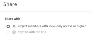
Public link creation in Autodesk Docs is off by default. This means that your recipient must own Autodesk Docs and be logged in to view or download a file you have shared. You’re presented with this option when sharing a file or folder by default. Note the disabled public link option (Anyone with this link).
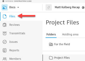
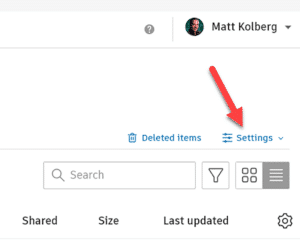
To enable public links, go to Doc and Files. Then click on Settings.
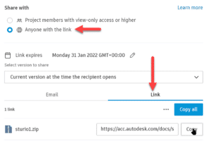
Once enabled, here is how the sharing form appears. The public link option is enabled, and the link can be copied and sent to anyone.
Autodesk is spending many resources getting their cloud system tweaked just right. Yet another version of the Desktop Connector has been made available. Read on to find out more.
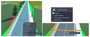
It’s relatively easy to create a custom component road assembly within an Infraworks model. But how does one save that custom assembly for use later? Read on to find out!
The answer depends on how you’d like it to be shared:
Export for use in other existing models.
Save for use when new models are created.
Saving the Assembly
First, to save a custom assembly, simply right click the component road and choose Add to Library. Choose a station to copy and give the new assembly a name. The new assembly will appear in the style palette.
Choose a station to copy and give the new assembly a name. The new assembly will appear in the style palette.
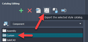
Export for Existing Models
The individual assembly cannot be exported, but the catalog can. Select the catalog, in this case, Custom, and click to export to a JSON file.
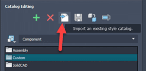
The JSON file can then be imported into a different existing model using the import button. The assembly will be available in the styles palette.
Save for Future Models
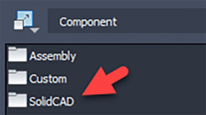
There is no “tool” for this, but if one copies the appropriate files from and to the correct locations, then it works just fine. The custom assembly files can be found in the model’s folder path.
…model.files\unver\Content\Styles\Component\ . Possibly in a Custom sub-folder.
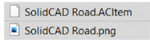
There will be 2 files for each assembly. A PNG image and a ACItem file.
Copy these two files to the Infraworks standard folder. Feel free to create a sub-folder here to place your custom assemblies. This folder will appear within Infraworks.
Many of our customers desire the ability to transform Civil 3D data between coordinate systems. This was challenging or impossible…until now! Read on…
It is available for Civil 3D 2019-2022. Read more about this extension here.
The Autodesk® PPK Survey Extension 2022 for Civil 3D® provides an interface for importing GPS data (in RINEX format) for analysis, reporting, and converting it to coordinate geometry points in an Autodesk Civil 3D drawing. Once installed, users can access the Autodesk PPK Survey Extension 2022 for Civil 3D commands via the Autodesk Civil 3D Toolbox.
We are excited to share with you the highlights of the latest Autodesk Desktop Connector update!
Enhancements are:
Folders Shared using Autodesk Drive are now visible on the desktop when using Desktop Connector.
When using Autodesk Collaboration for Civil 3D, an XML configuration file can be used to prevent a drawing’s reference template file from being uploaded when saving or dragging and dropping the drawing to Autodesk Docs.
AutoCAD 2022.1 will no longer create bak, dwl, dwl2 files when the dwg was opened from the workspace. For AutoCAD releases prior to 2022.1, Desktop Connector will add dwl and dwl2 files to the ignore list so they will no longer be uploaded.
In Autodesk Drive web, ‘My Data’ cannot be renamed or deleted. To match that behavior, Desktop Connector has removed those commands when right clicking on ‘My Data’.
Unnecessary “Checking Latest Version” dialog showing up during AutoCAD dwg compare workflow.
There have been significant changes to folder sharing. If you have folders shared, it is recommended to educate yourself on the new behavior.
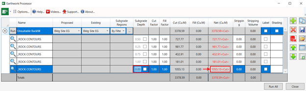
Earthworks Processor is a great tool in the CTC CIM Project suite for automating hours of surface creation and manipulation for the purpose of calculating dynamic and accurate earthworks quantities. With the use of a finished grade surface, existing grade surface, and simple closed polyline “regions”, Earthworks Processor will create 6 different surfaces including a stripping surface, earthworks volumes surface, and a subgrade surface. As well as offer bound volume outputs in the form of tables and labels.
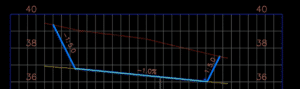
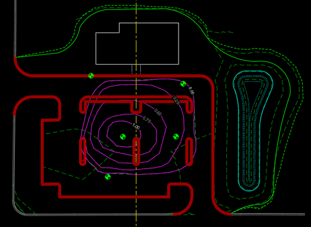
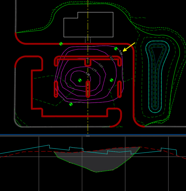
Today I want to talk about an alternative use for EWP. A dynamic way to calculate volumes and map profiles of points of interest from borehole data. This data could be anything from tops or bottoms of contaminant plumes to bedrock mapping, to volumes of loam that cannot be used for backfill. Borehole data of such points of interest is generally represented in depths from the existing surface, not elevations, and it can be tedious to get correct elevations mapped out.
EWP only requires the existing surface and some closed regions identifying depths of the unsuitable backfill (in this case). I have mapped this out as depth contours in the capture below.
These depth contours are derived from the borehole data, but without manually calculating, there is no efficient way to turn these depths into true elevations.
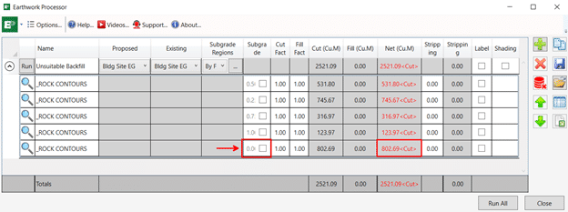
EWP can take these depths and run them through its processing to produce surfaces relative to the varying elevations of the existing surface as well as get you accurate volumes that will be dynamically updated as new borehole information is added to the design. In this scenario it’s the polyline region with the depth of 0 (or the extents of the unsuitable fill) that will give us the volume of unsuitable fill that we are looking for.
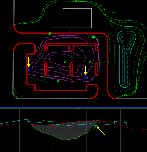
This whole process from mapped estimated depth contour polylines to dynamic volumes and surfaces is about 5 mins. The power and ROI of EWP is even more apparent when additional borehole information is added. Depth contours are modified, and EWP is rerun, and surfaces and volumes are updated in seconds.
I would like to acknowledge Jae Kwon, another Civil Technical Consultant on our SolidCAD team for this alternative EWP workflow. I hope this blog post earned your time today and helps you save time on future projects as well.
We are pleased to announce that our partner CTC Software released Civil 3D CIM Project Suite, version 22.0.3. It is now released and can be accessed on the CTC website.
Below are release notes:
22.0.3
9/17/2021
CIM Project Suite
Auto Grader
Bug Fix
Fixed an issue where “split points” in parent feature lines were causing an error. Fixed an issue where creating parallel child lines with a specified station range caused unexpected results. Fixed an issue where inward and outward offsetting was giving unexpected results. Fixed an issue where perpendicular child feature lines were not creating at the user-defined station values. Misc. user interface improvements.
22.0.3
9/17/2021
CIM Project Suite
Corridor Mapper
Bug Fix
Fixed an issue where corridors with disabled regions were causing the app to fail. Fixed an issue in how the app dealt with corridors containing previously mapped targets.
22.0.3
9/17/2021
CIM Project Suite
Corridor Splitter
New Features
Added interactive region selection and graphical highlighting, providing a much more intuitive app workflow.
22.0.3
9/17/2021
CIM Project Suite
Earthwork Processor
Bug Fix
Fixed an issue where the region offset command would not work on very small region objects.
22.0.3
9/17/2021
CIM Project Suite
Label Genie
Bug Fix
Fixed an issue where pipe networks could no longer be labelled.
22.0.3
9/17/2021
CIM Project Suite
Pipe Planner
Bug Fix
Fixed an issue where part elevations were not updating in the app after applying changes to the drawing. Fixed an issue where part elevations were not updating when importing external spreadsheets. Fixed an issue where pipe lengths for the pipe depth at interval property were not calculating correctly. Fixed an issue where parts of the same name, but in different pipe networks, were not allowed by the app. Fixed an issue where the structure rotation angle was incorrectly rounding.
Label Genie can save you a ton of time by creating all sorts of useful labels quickly. Here’s 15 examples that you can use right now.
Descriptions of the settings are included, but to really get up and running quickly Label Genie template files and the sample DWGs have been made available as well. Simply copy the .lg files into %AppData%\CTC\Label Genie then open up Label Genie. They will then show up in the dropdown box in the Label Genie template section.
If the labels you are creating are for design purposes, you may want to set their layers to a non-plotting style that you can ignore, or a layer that you can just freeze without affecting others.
Labelling for Corridor Design (*Corridor Design.dwg)
1. Label Assemblies (*Assembly Name.lg)
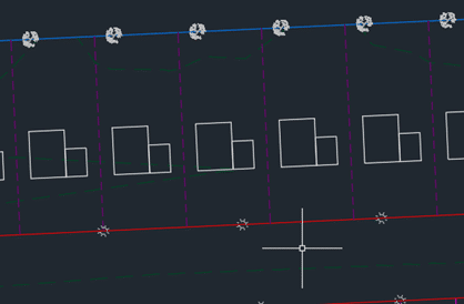
Make it easier to which assembly is which at a glance by label their names. The labelling is done with a field, so that if the assembly name changes, a simple regen will update the label.
Type = Multiline Text
Anchor Object = Assemblies (Layer filter = *)
Formatting, contents = (Assemblies).(Name)
Formatting, Y offset = -4
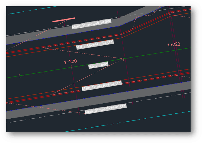
2. Label Alignment Names (*Alignment Name.lg)
When doing corridor work, we may want to see alignment names at a glance. This is especially true if setting up a lot of labels with the Corridor Mapper, for instance. Label the alignment names at regular intervals, oriented with the lines to avoid having to check the property palette constantly.
Label Type = Multiline Text
Anchor Object = Alignments (Layer filter = *)
Anchor Point = Vertices (Interval = 100, rest unchecked)
Formatting, contents = (Alignments).(Name)
Formatting, orientation = To Objects
Formatting, Y Offset = -0.5
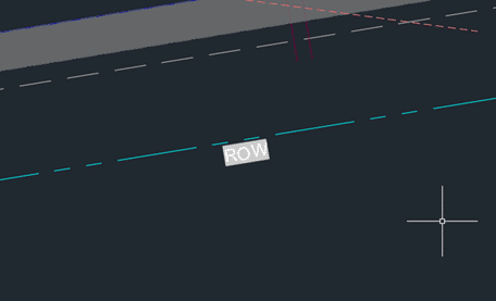
3. Label Feature Line and Polyline Layers (*Feature Line Layer.lg / Polyline Layer.lg)
Continuing the theme of adding some labels to corridor target objects, we can label feature line (and polylines) layer names at intervals. For feature lines, you may want to switch the Contents to the feature line’s name instead of the layer name – depending on how you like to use feature lines.
Label Type = Multiline Text
Anchor Object = Feature Lines (Layer filter = *)
Anchor Point = Vertices (Interval = 100, rest unchecked)
Formatting, contents = (Feature Lines).(Layer)
Formatting, orientation = To Objects
Formatting, Y Offset = -0.5
If you have a lot of polylines for use for horizontal target condition subassemblies, you can label those as well, to make it easier to see what layer names they have. They tend to be shorter, so instead of intervals, midpoints might be more appropriate.
Label Type = Multiline Text
Anchor Object = Feature Lines (Layer filter = *)
Anchor Point = Vertices (Interval = 100, rest unchecked)
Formatting, contents = (Feature Lines).(Layer)
Formatting, orientation = To Objects
Formatting, Y Offset = -0.5
Labelling for Presentation (*Presentation.dwg)
Sometimes, we need to fill in some objects in the drawing for conceptual presentation. At the conceptual stage, we can forego precise placement and mass populate objects such as trees, lights, and structures quickly. These objects, in turn, can be exported to InfraWorks for even greater visual impact.
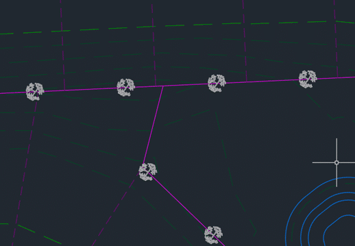
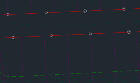
4. Place Tree Blocks at Back of Lots (*Place Trees.lg)
First, we can place some trees at an interval at the back lot line.
Formatting, rotation / x offset / y offset = 0 / 0 / -8
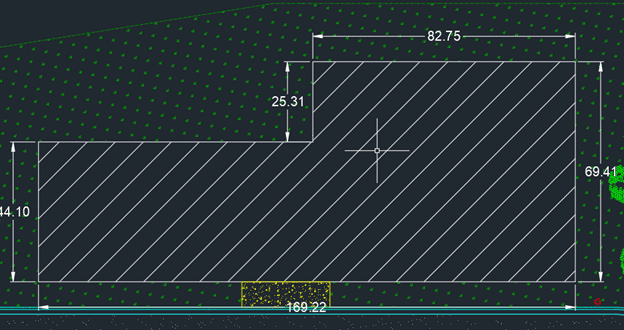
9. Measure Areas (*measure areas.lg)
Next, we generate area quantity labels for various hatching in the drawing. Note that labels are created in the centroids of hatches. This means that if you have an “L” shaped hatch, such as the grass in this drawing, the label may end up being outside the hatch. Some manual repositioning may be required.
Label Type = MultilineText
Anchor Object = Hatches (layer filter = *)
Anchor Point = Centroid
View Type = Plan
Formatting contents =
(Hatches).(Layer)
<New Line>
(Hatches).(Area)
Field customization: Format = Decimal, Precision = 0.0, Suffix = sq. m.
Formatting, Style = Annotative
Formatting, display width = 12
More Labelling Tips On the Way
That concludes the first 9 of the 15 time-saving shortcuts using the CTC Label Genie. It can help us quickly generate labels that can help us find the design information we need, place blocks to flesh out a conceptual design drawing, and dimension and measure various objects.
Keep an eye out for Part 2, where we cover locating points and objects, as well as communication key surface information.